딥러닝 이야기 / Recurrent Neural Network (RNN) / 4. Seq2Seq 모델을 이용한 기계 번역

작성일: 2022.09.12
시작하기 앞서 틀린 부분이 있을 수 있으니, 틀린 부분이 있다면 지적해주시면 감사하겠습니다.
이전글에서는 sequence-to-sequence (seq2seq) 모델과 attention 메커니즘 예시와 scheduled sampling에 대해 살펴보았습니다.
이번글에서는 GRU 모델을 이용하여 Tatoeba Project의 English-French 문장 쌍 데이터를 가지고 기계 번역 모델을 학습하고, Bahdanau attention mechanism (바다나우 어텐션)과 scheduled sampling을 적용 해보겠습니다.
본 코드는 영어 문장을 프랑스어로 번역하는 모델이며, 구현은 python의 PyTorch를 이용하였습니다. 그리고 모델을 학습하면서 training set과 test set의 loss의 변화와 더불어, 각종 지표 (PPL, BLEU, NIST), attention score, 기계 번역 결과 샘플도 살펴보겠습니다.
그리고 seq2seq 모델, attention, scheduled sampling에 대한 설명은 이전글을 참고하시기 바랍니다.
그리고 학습을 위한 코드는 GitHub에 올려놓았으니 아래 링크를 참고하시기 바랍니다(본 글에서는 모델의 구현에 초점을 맞추고 있기 때문에, 데이터 전처리 및 학습을 위한 전체 코드는 아래 GitHub 링크를 참고하시기 바랍니다).
그리고 텍스트를 토큰화 하기 위해 사용한 토크나이저는 word tokenizer를 구현하여 사용하였습니다.
물론 현재는 unknown 토큰 문제를 해결하기 위해 Word2Vec 글에서 설명한 byte-pair-encoding (BPE) 같이 subword 기반의 토크나이저가 많이 사용되지만, 본 글에서는 attention 모델이 결과를 예측하기 위해 어떠한 단어에 집중을 했는지 그 score를 보기 위해서 단어 기반의 토크나이저를 선택하였습니다.
여담으로 PyTorch의 유명한 seq2seq 기계 번역 모델 튜토리얼이 있습니다. 이 튜토리얼에서는 Bahdanau attention이 아닌 다른 attention 기법으로 구현 되어있습니다.
다른 attention 기반의 코드를 보고싶다면 튜토리얼 링크를 참고하시기 바랍니다. PyTorch 튜토리얼 코드는 batch 학습을 하지 않기 때문에 시간이 오래 걸린다는 단점이 있습니다.
오늘의 컨텐츠입니다.
- GRU 기계 번역 모델
- Attention 모듈
- 기계 번역 모델 학습
- 기계 번역 모델 학습 결과
본 코드에서 구현한 Bahdanau Attention (바다나우 어텐션)과 scheduled sampling에 대한 논문은 아래 링크에 달아놓겠습니다.
Attention과 Scheduled Sampling을 이용한 GRU 기계 번역 모델
”
여기서는 기계 번역을 위한 GRU 코드를 살펴보겠습니다. 코드는 PyTorch로 작성 되었으며, source 문장을 encoder를 통해 represent 한 후, 이를 바탕으로 decoder에 target 문장을 넣어 학습합니다. 만약 Bahdanau attention을 사용한다면 encoder 결과를 attention하는 데 사용합니다.
class Encoder(nn.Module):
    def __init__(self, config, tokenizer, device):
        super(Encoder, self).__init__()
        self.pad_token_id = tokenizer.pad_token_id
        self.vocab_size = tokenizer.vocab_size
        self.hidden_size = config.hidden_size
        self.num_layers = config.num_layers
        self.dropout = config.dropout
        self.device = device

        self.embedding = nn.Embedding(self.vocab_size, self.hidden_size, padding_idx=self.pad_token_id)
        self.gru = nn.GRU(input_size=self.hidden_size,
                            hidden_size=self.hidden_size,
                            num_layers=self.num_layers,
                            batch_first=True,
                            dropout=self.dropout,
                            bidirectional=True)
        self.dropout_layer = nn.Dropout(self.dropout)


    def init_hidden(self):
        h0 = torch.zeros(self.num_layers*2, self.batch_size, self.hidden_size).to(self.device)
        return h0


    def forward(self, x):
        self.batch_size = x.size(0)
        h0 = self.init_hidden()

        x = self.embedding(x)
        x = self.dropout_layer(x)
        x, hn = self.gru(x, h0)
        hn = hn.view(2, -1, self.batch_size, self.hidden_size)
        hn = torch.sum(hn, dim=0)
        return x, hn


class Decoder(nn.Module):
    def __init__(self, config, tokenizer, device):
        super(Decoder, self).__init__()
        self.pad_token_id = tokenizer.pad_token_id
        self.vocab_size = tokenizer.vocab_size
        self.hidden_size = config.hidden_size
        self.num_layers = config.num_layers
        self.dropout = config.dropout
        self.is_attn = config.is_attn
        self.device = device
        if self.is_attn:
            self.attention = Attention(self.hidden_size)
        self.input_size = self.hidden_size * 2 if self.is_attn else self.hidden_size

        self.embedding = nn.Embedding(self.vocab_size, self.hidden_size, padding_idx=self.pad_token_id)
        self.gru = nn.GRU(input_size=self.input_size,
                            hidden_size=self.hidden_size,
                            num_layers=self.num_layers,
                            batch_first=True,
                            dropout=self.dropout)
        self.dropout_layer = nn.Dropout(self.dropout)
        self.relu = nn.ReLU()
        self.fc = nn.Linear(self.hidden_size, self.vocab_size)


    def forward(self, x, hidden, enc_output, mask):
        self.batch_size = x.size(0)
        score = None

        x = self.embedding(x)
        if self.is_attn:
            enc_output, score = self.attention(self.relu(enc_output), self.relu(hidden[-1]), mask)
            x = torch.cat((x, enc_output.unsqueeze(1)), dim=-1)
        x = self.dropout_layer(x)
        x, hn = self.gru(x, hidden)
        x = self.fc(self.relu(x))
        return x, hn, score
위 코드에서 나오는 config 부분은 GitHub 코드에 보면 config.json이라는 파일에 존재하는 변수 값들을 모델에 적용하여 초기화 하는 것입니다.
Encoder
- 4번째 줄: Vocab 중 pad token id 값.
- 5번째 줄: 토크나이저의 vocab size.
- 6번째 줄: GRU 모델 hidden dimension.
- 7번째 줄: GRU 모델 레이어 수.
- 8번째 줄: GRU 모델 dropout 비율.
- 11 ~ 18번째 줄: Embedding 레이어, GRU 모델, dropout layer 선언.
- 21 ~ 23번째 줄: GRU hidden state 초기와 함수.
- 26 ~ 35번째 줄: Source 문장(본 코드에서는 영어 문장)이 학습 시 거치는 부분.
- 34번째 줄: Encoder는 bidirectional 모델이므로, 단방향 GRU인 decoder보다 hidden state 결과가 2배가 많음. 따라서 decoder에 hidden state를 넣어주기 위해서는 차원을 맞춰줘야함. 따라서 각 레이어별 forward, backward hidden state 결과를 더해주어 하나의 hidden으로 취급.
Decoder
- 42번째 줄: Vocab 중 pad token id 값.
- 43번째 줄: 토크나이저의 vocab size.
- 44번째 줄: GRU 모델 hidden dimension.
- 45번째 줄: GRU 모델 레이어 수.
- 46번째 줄: GRU 모델 dropout 비율.
- 47번째 줄: Attention 사용 여부.
- 49 ~ 50번째 줄: Attention 사용하는 경우 Attention 모듈 정의.
- 51번째 줄: Attention을 사용할 경우 decoder input 차원은 사용안할 때 비해 2배가 커짐(Attention 결과를 다음 decoder input에 대해 concatenate하여 들어가기 때문).
- 53 ~ 59번째 줄: Embedding 레이어, GRU 모델, dropout layer 선언.
- 61번째 줄: 다음 단어를 예측해야하므로 vocab size의 크기만큼 내어주는 fully-connected layer 선언.
- 64 ~ 75번째 줄: Target 문장(본 코드에서는 프랑스어 문장)이 학습 시 거치는 부분.
- 69 ~ 71번째 줄: Attention 사용 시 거치는 부분. Target input에 concatenate 하기 때문에 attention 사용 하지 않는 모델 대비 차원이 2배가 큼.
- 75번째 줄: Attention score도 결과와 같이 반환.
”
위의 GRU 기반 seq2seq 모델에서 attention을 사용할건지 여부를 선택할 수 있었습니다. 만약 attention을 선택하게 된다면 아래의 attention 모듈에 GRU encoder의 output과 deccoder의 이전 output이 들어가게 됩니다.
class Attention(nn.Module):
    def __init__(self, hidden_size):
        super(Attention, self).__init__()
        self.hidden_size = hidden_size
        self.enc_dim_changer = nn.Sequential(
            nn.Linear(self.hidden_size*2, self.hidden_size),
        )
        self.enc_wts = nn.Sequential(
            nn.Linear(self.hidden_size, self.hidden_size)
        )
        self.dec_wts = nn.Sequential(
            nn.Linear(self.hidden_size, self.hidden_size),
            nn.ReLU(),
            nn.Linear(self.hidden_size, self.hidden_size)
        )
        self.score_wts = nn.Linear(self.hidden_size, 1)
        self.tanh = nn.Tanh()
        self.relu = nn.ReLU()


    def forward(self, enc_output, dec_hidden, mask):
        enc_output = self.enc_dim_changer(enc_output)
        score = self.tanh(self.enc_wts(self.relu(enc_output)) + self.dec_wts(dec_hidden).unsqueeze(1))
        score = self.score_wts(score)
        score = score.masked_fill(mask.unsqueeze(2)==0, float('-inf'))
        score = F.softmax(score, dim=1)

        enc_output = torch.permute(enc_output, (0, 2, 1))
        enc_output = torch.bmm(enc_output, score).squeeze()
        return enc_output, score
Attention
위 코드에서 나오는 config 부분은 GitHub 코드에 보면 config.json이라는 파일에 존재하는 변수 값들을 모델에 적용하여 초기화 하는 것입니다.
- 5번째 줄: Encoder는 bidirectional GRU이므로 decoder 차원을 맞춰주기 위해서 차원의 크기를 절반으로 줄이는 linear layer 선언.
- 8 ~ 15번째 줄: Encoder의 output과 decoder의 output이 거치게 되는 linear layer 선언.
- 16번째 줄: Encoder의 각 sequence 별 attention score를 내어줘야 하므로 차원을 hidden dim → 1로 바꿔주는 layer 선언.
- 21 ~ 30번째 줄: Attention 모듈 학습 시 거치는 부분.
- 25번째 줄: Attention score를 내어주기 위해 softmax 하기 전, encoder 데이터 중 pad token에 대해 masking하는 작업(-inf로 선언 시, softmax 결과가 0).
- 29번째 줄: Attention score를 encoder output에 곱해주어 weighted sum 하는 부분.
”
이제 기계 번역 모델 학습 코드를 통해 어떻게 학습이 이루어지는지 살펴보겠습니다. 아래 코드에 self. 이라고 나와있는 부분은 GitHub 코드에 보면 알겠지만 학습하는 코드가 class 내부의 변수이기 때문에 있는 것입니다. 여기서는 무시해도 좋습니다.
self.encoder = Encoder(self.config, self.src_tokenizer, self.device).to(self.device)
self.decoder = Decoder(self.config, self.trg_tokenizer, self.device).to(self.device)
self.criterion = nn.CrossEntropyLoss()
self.enc_optimizer = optim.Adam(self.encoder.parameters(), lr=self.lr)
self.dec_optimizer = optim.Adam(self.decoder.parameters(), lr=self.lr)

for epoch in range(self.epochs):
    for phase in ['train', 'test']:
        if phase == 'train':
            self.encoder.train()
            self.decoder.train()
        else:
            self.encoder.eval()
            self.decoder.eval()

        for i, (src, trg, mask) in enumerate(self.dataloaders[phase]):
            batch = src.size(0)
            src, trg = src.to(self.device), trg.to(self.device)
            if self.config.is_attn:
                mask = mask.to(self.device)
            self.enc_optimizer.zero_grad()
            self.dec_optimizer.zero_grad()

            with torch.set_grad_enabled(phase=='train'):
                enc_output, hidden = self.encoder(src)

                teacher_forcing = True if random.random() <= self.config.teacher_forcing_ratio else False
                decoder_all_output = []
                for j in range(self.max_len):
                    if teacher_forcing or j == 0 or phase == 'test':
                        trg_word = trg[:, j].unsqueeze(1)
                        dec_output, hidden, _ = self.decoder(trg_word, hidden, enc_output, mask)
                        decoder_all_output.append(dec_output)
                    else:
                        trg_word = torch.argmax(dec_output, dim=-1)
                        dec_output, hidden, _ = self.decoder(trg_word.detach(), hidden, enc_output, mask)
                        decoder_all_output.append(dec_output)

                decoder_all_output = torch.cat(decoder_all_output, dim=1)
                loss = self.criterion(decoder_all_output[:, :-1, :].reshape(-1, decoder_all_output.size(-1)), trg[:, 1:].reshape(-1))
                if phase == 'train':
                    loss.backward()
                    self.enc_optimizer.step()
                    self.dec_optimizer.step()
학습에 필요한 것들 선언
먼저 위에 코드에서 정의한 모델을 불러오고 학습에 필요한 loss function, optimizer 등을 선언하는 부분입니다.
- 1 ~ 5번째 줄: Loss function, encoder, decoder 모델 선언 및 각각의 optimizer 선언.
기계 번역 모델 학습
다음은 기계 번역 모델 학습 부분입니다. 코드상에서는 5 ~ 26번째 줄에 해당하는 부분입니다.
- 19 ~ 20번째 줄: Attention 모델일 시 encoder에 들어가는 source 문장 토큰 중, pad token을 masking 하기위한 mask를 device에 올림.
- 29 ~ 37번째 줄: Teacher forcing (교사 강요)로 학습 하지 않을 시, scheduled sampling 방법으로 학습 하는 부분(Attention을 위해서 decoder에 들어가는 문장은 한 단어씩 들어가게 구성).
- 40 ~ 44번째 줄: Loss를 계산하고 모델을 업데이트 하는 부분.
”
먼저 본 글에서는 4가지 모델의 결과를 비교합니다.
- Attention을 사용한 모델
- Scheduled sampling과 attention을 사용한 모델
- Attention을 사용하지 않은 모델
- Scheduled sampling을 사용했지만 attention을 사용하지 않은 모델
Training Set Loss History

Training set loss history
Test Set Loss History

Test set loss history
- Attention을 사용한 모델: 0.3367
- Scheduled sampling과 attention을 사용한 모델: 0.3509
- Attention을 사용하지 않은 모델: 0.3366
- Scheduled sampling을 사용했지만 attention을 사용하지 않은 모델: 0.3491
Test Set Perplexity (PPL) History

Test set PPL history
- Attention을 사용한 모델: 1.4003
- Scheduled sampling과 attention을 사용한 모델: 1.4203
- Attention을 사용하지 않은 모델: 1.4002
- Scheduled sampling을 사용했지만 attention을 사용하지 않은 모델: 1.4178
Test Set BLEU-2 History

Test set BLEU-2 history
- Attention을 사용한 모델: 0.5789
- Scheduled sampling과 attention을 사용한 모델: 0.5646
- Attention을 사용하지 않은 모델: 0.5735
- Scheduled sampling을 사용했지만 attention을 사용하지 않은 모델: 0.5656
Test Set BLEU-4 History
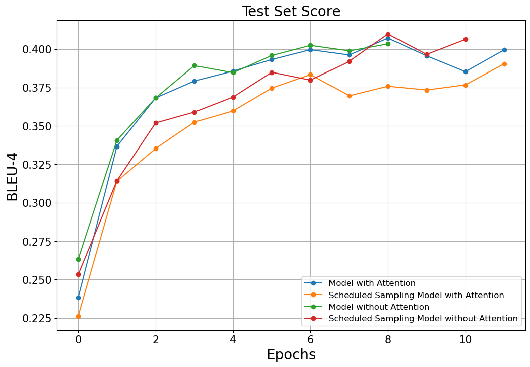
Test set BLEU-4 history
- Attention을 사용한 모델: 0.3996
- Scheduled sampling과 attention을 사용한 모델: 0.3834
- Attention을 사용하지 않은 모델: 0.3893
- Scheduled sampling을 사용했지만 attention을 사용하지 않은 모델: 0.3849
Test Set NIST-2 History

Test set NIST-2 history
- Attention을 사용한 모델: 6.8475
- Scheduled sampling과 attention을 사용한 모델: 6.6922
- Attention을 사용하지 않은 모델: 6.8016
- Scheduled sampling을 사용했지만 attention을 사용하지 않은 모델: 6.7098
Test Set NIST-4 History

Test set NIST-4 history
- Attention을 사용한 모델: 7.1627
- Scheduled sampling과 attention을 사용한 모델: 7.0052
- Attention을 사용하지 않은 모델: 7.1178
- Scheduled sampling을 사용했지만 attention을 사용하지 않은 모델: 7.0177
기계 번역 결과 샘플
그리고 아래는 예측한 몇 개의 샘플입니다.
- Attention을 사용한 모델
# Sample 1
src : when i was your age , i had a girlfriend .
gt  : lorsque j'avais votre age , j'avais une petite amie .
pred: lorsque j'avais votre age , j'avais une petite amie .

# Sample 2
src : he gave me some money .
gt  : il me donna un peu d'argent .
pred: il me donna un peu d'argent .

# Sample 3
src : please answer all the questions .
gt  : repondez a toutes les questions , s'il vous plait .
pred: repondez a toutes les questions , s'il vous plait .

Attention score
Attention이 source 문장과 target 문장의 순서에 맞게 잘 align되어 참고하고 있는 것을 확인할 수 있습니다.
- Scheduled sampling과 attention을 사용한 모델
# Sample 1
src : i'm in love with you and i want to marry you .
gt  : je suis amoureuse de toi et je veux me marier avec toi .
pred: je vous amoureux de toi et je veux vous epouser . toi .

# Sample 2
src : what's really going one here ?
gt  : que se passe-t-il vraiment ici ?
pred: que se passe-t-il, ici ?

# Sample 3
src : we do need your advice .
gt  : il nous faut ecouter vos conseils .
pred: nous nous faut que tes conseils .

Attention score
Scheduled sampling을 사용한 모델에 대해서도 attention이 source 문장과 target 문장의 순서에 맞게 잘 align되어 참고하고 있는 것을 확인할 수 있습니다.
- Attention을 사용하지 않은 모델
# Sample 1
src : tom asked mary for some help .
gt  : tom a demande a mary de l'aider .
pred: tom demande demande a mary de l'aide .

# Sample 2
src : you see what i mean ?
gt  : tu vois ce que je veux dire ?
pred: tu vois ce que je veux dire ?

# Sample 3
src : i haven't talked to you in a while .
gt  : je ne t'ai pas parle depuis un bon moment .
pred: je n'ai vous pas parle pendant un moment moment .
- Scheduled sampling을 사용했지만 attention을 사용하지 않은 모델
# Sample 1
src : let's take a little break .
gt  : faisons une petite pause .
pred: faisons une pause pause .

# Sample 2
src : they live on the [UNK] floor of this [UNK] .
gt  : ils vivent au [UNK] etage de ces [UNK] .
pred: ils vivent au sujet de de ce sujets .

# Sample 3
src : tom doesn't understand why mary is so popular .
gt  : tom ne comprend pas pourquoi marie est si populaire .
pred: tom ne comprend pas pourquoi mary est si populaire .
지금까지 GRU 통한 Tatoeba Project English-French 데이터를 이용하여 기계 번역 모델을 구현해보았습니다.
학습 과정에 대한 전체 코드는 GitHub에 있으니 참고하시면 될 것 같습니다.


